Hands-On Machine Learning -- SVM

SVM 线性分类器
非线性 SVM 分类器
用 SVM 做回归

SVM 线性分类器

本例使用 iris 数据集来做分类。

# 导入模块 
import numpy as np
import matplotlib.pyplot as plt

导入数据

from sklearn import datasets
iris = datasets.load_iris()

============== ==== ==== ======= ===== ====================
                Min  Max   Mean    SD   Class Correlation
============== ==== ==== ======= ===== ====================
sepal length:   4.3  7.9   5.84   0.83    0.7826
sepal width:    2.0  4.4   3.05   0.43   -0.4194
petal length:   1.0  6.9   3.76   1.76    0.9490  (high!)
petal width:    0.1  2.5   1.20   0.76    0.9565  (high!)
============== ==== ==== ======= ===== ====================

上面是数据集的概要，每个样本包含 4 个属性，此处只选择了相关系最高的两个。

X = iris['data'][:, (2, 3)]
y = (iris['target'] == 2).astype(np.float64)

划分训练集和测试集

from sklearn.model_selection import train_test_split

X_train, X_test, y_train, y_test = train_test_split(X, y, test_size=0.3)

训练 SVM 分类器

SVM 分类器对数据尺度非常敏感，因此在数据预处理阶段，要对样本属性值进行标准化操作，可以使用 StandardScaler 轻松完成此操作。

使用 SVM 对线性可分的样本进行分类，可以使用 LinearSVC，也可以使用 SVC(kernel='linear')，但是后者的速度要慢很多。

现实场景下，完全线性可分的数据很少，SVM 的软间隔用来完成近似线性可分的样本集的分类。LinearSVC 中的 C 参数表示惩罚程度，此处即对落入 margin 内样本的惩罚程度。C 越大，当样本落入 margin 中时，损失就越大，因此为了让的样本不落入 margin 中，相应地 margin 也就越窄。

这里 hinge 损失函数是 SVM 默认的损失函数。

from sklearn.svm import LinearSVC
from sklearn.pipeline import Pipeline
from sklearn.preprocessing import StandardScaler

svm_clf = Pipeline((
    ('scaler', StandardScaler()),
    ('linear_svc', LinearSVC(C=1, loss="hinge"))
))

svm_clf.fit(X_train, y_train)

评估性能

from sklearn.metrics import precision_score, recall_score

y_pred = svm_clf.predict(X_test)

precision_score(y_test, y_pred), recall_score(y_test, y_pred)

准确率和召回率：

(0.8571428571428571, 0.9230769230769231)

观察决策面（线）

import matplotlib.pyplot as plt

def plot_predictions(clf, axes):
    x1 = np.linspace(axes[0], axes[1], 100)
    x2 = np.linspace(axes[2], axes[3], 100)
    X1, X2 = np.meshgrid(x1, x2)
    X = np.vstack((X1.ravel(), X2.ravel())).T
    Y = clf.predict(X).reshape(X1.shape)
    plt.contourf(X1, X2, Y, cmap=plt.cm.brg, alpha=0.2)
    
plt.plot(X_test[y_test == 0, 0], X_test[y_test == 0, 1], 'rv')
plt.plot(X_test[y_test == 1, 0], X_test[y_test == 1, 1], 'go')

plot_predictions(svm_clf, [1, 7, 0, 3])

非线性 SVM 分类器

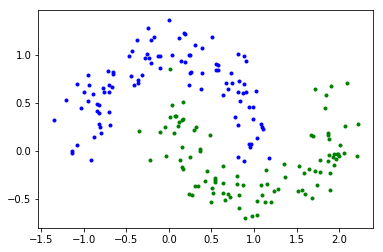
生成数据集

make_moons 用于生成呈半月形分布的两类样本，此处用它来生成样本。

from sklearn.datasets import make_moons
X, y = make_moons(n_samples=200, noise=0.15, random_state=42)

# 观察样本
plt.plot(X[:, 0][y==0], X[:, 1][y==0], 'b.')
plt.plot(X[:, 0][y==1], X[:, 1][y==1], 'g.')

## 划分训练集和测试集

from sklearn.model_selection import train_test_split

X_train, X_test, y_train, y_test = train_test_split(X, y, test_size=0.3)

训练分类器

这个数据集是线性不可分的，但可以样本增加属性，将其升至高维。在高维空间中能够找到一个超平面，将两类样本分开。

此处使用 PolynomialFeatures 来给样本增加属性，新增的属性值是原属性的四阶多项式。

from sklearn.pipeline import Pipeline
from sklearn.preprocessing import PolynomialFeatures
from sklearn.preprocessing import StandardScaler

ploy_svm_clf = Pipeline((
    ('poly_features', PolynomialFeatures(degree=4)),
    ('scaler', StandardScaler()),
    ('svm_clf', LinearSVC(C=1, loss="hinge"))
))

ploy_svm_clf.fit(X_train, y_train)

### 观察决策面（线）

plot_predictions(ploy_svm_clf, [-2, 3, -1, 1.5])

plt.plot(X_train[y_train == 1, 0], X_train[y_train == 1, 1], 'g.', alpha=0.4, label="train 1")
plt.plot(X_train[y_train == 0, 0], X_train[y_train == 0, 1], 'rx', alpha=0.4, label="train 0")

plt.plot(X_test[y_test == 1, 0], X_test[y_test == 1, 1], 'gv', label="test 1")
plt.plot(X_test[y_test == 0, 0], X_test[y_test == 0, 1], 'r^', label="test 0")
plt.legend(loc="upper right")

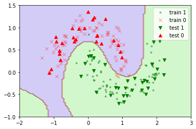
可以看到测试集被完全正确地分类。

使用多项式核

前面解决线性不可分问题的方法是采用 PolynomialFeatures 给样本增加额外的属性。SVM 分类器可以用核方法来处理线性不可分问题，多项式核将样本属性值做多项式变换，使原来线性不可分样本转变为线性可分。

下面示例这里使用多项式核来进行分类，这里用到了 SVC 类，它有以下重要参数：

kernel='poly' 表明使用多项式核
degree=3 表示最高为 3 阶
coef0 用于控制分类器对高阶项的偏重，此值越大越偏向于高阶。

#### 训练分类器

from sklearn.svm import SVC

poly_kernel_svm_clf = Pipeline((
    ('scaler', StandardScaler()),
    ('svm_clf', SVC(kernel='poly', degree=3, coef0=1, C=5))
))

poly_kernel_svm_clf.fit(X_train, y_train)

用 SVM 做回归

SVM 还可以用来做回归，只需要在分类的思想上稍作变换，即让尽可能多的样本落在 margin 中，同时让 margin 尽可能窄。

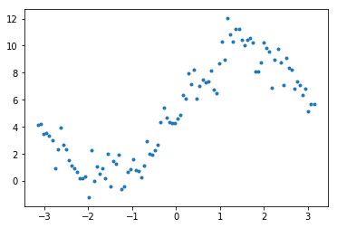
生成数据

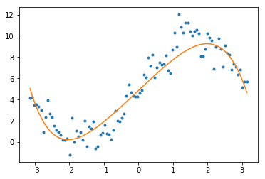
x = np.linspace(-np.pi, np.pi, 100);
y = 5 * np.sin(x) + 5 + np.random.randn(x.shape[0])

plt.plot(x, y, '.')

使用线性回归

上面生成的数据显然不是线性的，可以通过将样本做多项式变换，就可以使用 LinearSVR 来做线性回归了。

LinearSVR 的 epsilon 参数用于控制 margin 的宽度，这个值越小 margin 也就越小。

from sklearn.svm import LinearSVR

X = x.reshape(x.shape[0], 1)

svm_reg = Pipeline((
    ('poly', PolynomialFeatures(degree=7)),
    ('scaler', StandardScaler()),
    ('svm_clf', LinearSVR(epsilon=1))
))

svm_reg.fit(X, y)

y_pred = svm_reg.predict(X)

plt.plot(x, y, '.')
plt.plot(x, y_pred, '-')

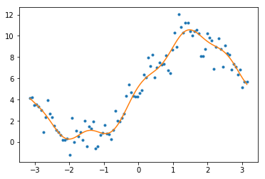
使用多项式核

也可以使用 SVR 利用其自身具备的核函数做非线性变换，来完成对非线性样本的回归。

当样本较大的时候，比如大于 1000 个，如果使用多项式核，SVR 就已经变得很慢了。此处使用默认的 rbf 核，稍快一些。

这里的参数 C 表示对误差的惩罚度，如果此值很小，常常会欠拟合，如果此值太大可能会过拟合。

from sklearn.svm import SVR

X = x.reshape(x.shape[0], 1)

poly_svm_reg = SVR(C=1, epsilon=0.01)
poly_svm_reg.fit(X, y)

y_pred = poly_svm_reg.predict(X)

plt.plot(x, y, '.')
plt.plot(x, y_pred, '-')